Linear Regression

Linear regression is the simplest method for regression analysis. With current state of machine learning and deep learning, we might often overlook linear regression, but it remains a popular method in practice. For instance, a linear regression model can be used to predict the sale price for an apartment from its properties after being trained on data about housing price. In this article, we're going through the formulation of linear regression and implement it from scratch in Python.

Formulation

Problem statement

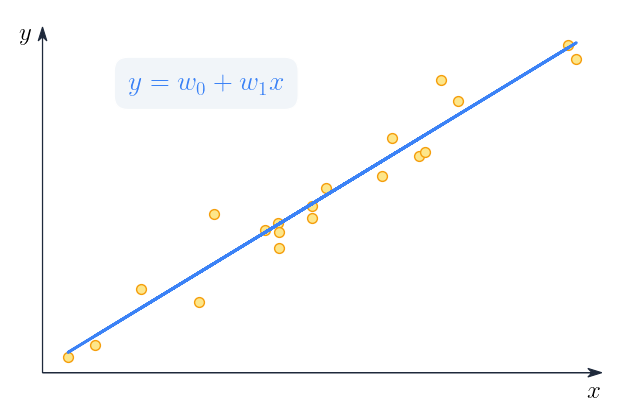
Linear regression is a supervised learning method that learns to model a dependent variable $y$ as a function of some independent variables, a.k.a, features, by finding the straight line that best fits the data. The data for linear regression comes as input/output pairs

where each input sample $\mathbf{x}_i$ is a vector of $p$ features, and the ouput $y_i$ is scalar-valued. In the simplest case, $p = 1$, i.e., the input has one feature, linear regression is like to drawing a straight trend line in a scatter plot. In general, however, $p > 1$ in which case the linear regression problem is analogous to fitting a hyperplane to a scatter points in $p + 1$ dimensional space.

Generally, the equation for linear regression for each data point iswhere $w_j$ is the coefficient of the model. The first coefficient $w_0$ is often called the *intercept* of the model. $\epsilon$ is the irreducable error that cannot be expressed by our model. As a side note, other people might denote the coefficient as $\beta_j$.

Since we have $N$ data points, the equation is often written in matrix form

where $X$ is the matrix of input data, and $\mathbf{W}$ is the coefficient matrix, or the weight matrix. You might have realized that there is something off about this equation. $X$ is of dimension $(N, p)$, while $\mathbf{W}$ is of the dimension $(p+1,)$; hence, matrix multiplication won't work here. To solve this issue, we can insert a constant $1$ as the first column of the matrix $\mathbf{X}$. And now our matrices look like followings

Fitting a linear regression model is all about finding the best weights $\mathbf{W}$ that best model $y$ as a function of the input features. While we might never find the "true" weights, we can estimate them. We are going to look into two methods for estimating the weights below. But first, let's look at the loss function for our linear regression model.

Loss function

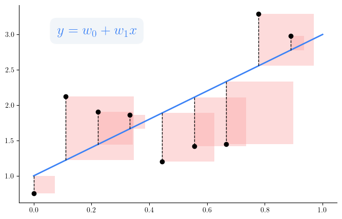
The loss function quantifies how good or bad our linear regression model is. To train the model, we employ the mean squared error (MSE) as our loss function.

We add a constant $\frac{1}{2}$ to the equation above to simplify the calculation of the gradient of this loss function, as shall be shown below. The square of the errors give more weight to points that are further from the regression line, thus, punishing more the outliners.

The optimal set of weights $\mathbf{\hat{W}}$ is the one that minize the loss function.

Our MSE loss function is a convex function; hence, we can find the optimal weights that minize the loss using methods such as Ordinary Least Squares (OLS) or Gradient Descent (GD).

Parameter estimation with Ordinary Least Squares

Let's look closer at the loss function

Since the loss function is convex, the optimum solution lies at gradient zero. So now we derive the gradient of the loss function w.r.t to $\mathbf{W}$Solve this equation equals to $0$, we getIf you're still mathematically curious, we can use the Gauss-Markov theorem to prove that the set of coefficients $\mathbf{W}$ obtained in the equation above is optimal.

Parameter estimation with Gradient Descent

Again, as the MSE loss function is a convex function; GD can have a chance to find the optimal minimum. Let's modify the equation for the gradient a bit

Having devised the gradient of our loss function, the update equation of the GD algorithm is

where $\eta$ is the learning rate.

Assumptions of Linear Regression model

For completeness of the topic, we list several assumptions made by the linear regression model. It is, however, worth to note that in machine learning, we often care about how well our model generalizes on unseen data rather than which assumptions it makes.

Implementation in Python

I hope that at this point you can convince yourself that implementing linear regression in Python is simple. Indeed, the main work is to implement the estimation of the weights $\mathbf{W}$.

import jax.numpy as jnp
from jax import random

class LinearRegression():

  def __init__(self, seed=0, gradient_descent=True, lr=0.01, n_iterations=100):
    self.gradient_descent = gradient_descent
    self.lr = lr
    self.n_iterations = n_iterations

    self._key = random.PRNGKey(seed)

  def _initialize_weights(self, X, y):
    N, m = X.shape
    self.W = random.uniform(self._key, shape=(m,), minval=-1 / N, maxval=1 / N)

  def fit(self, X, y):
    X = jnp.insert(X, 0, 1, axis=1)
    self._initialize_weights(X, y)
    if self.gradient_descent:
        for _ in range(self.n_iterations):
            y_pred = X.dot(self.W)
            grad_w = (y_pred - y).dot(X)
            self.W = self.W - self.lr * grad_w
    else:
        # Least-square to estimate model's parameters
        X_T_inv = jnp.linalg.inv(jnp.dot(X.T, X))
        self.W = X_T_inv.dot(X.T).dot(y)

  def predict(self, X):
    # insert constant 1 at the beginning of each row in X for the biases
    X = jnp.insert(X, 0, 1, axis=1)
    return jnp.dot(X, self.W)

As a small note, you probably see that in the code above, when computing the gradient of $\mathbf{W}$, the equation is $(\hat{\mathbf{y}} - \mathbf{y})\mathbf{X}$, i.e., there is no transpose. This is because $(\hat{\mathbf{y}} - \mathbf{y})$ is a column vector, and in Jax (or numpy), it is the same as its transpose.

Let's test our implementation by comparing the performance of our model with sklearn linear regression. To that end, we'll generate a synthetic regression dataset containing of $100$ samples, each has 5 features. To make it a bit more realistic, we add some noise to our data. We then train our model and sklearn model on this dataset, and compare their MSE loss on the test data.

# Create the dataset, and split into train/test
import jax.numpy as jnp
from sklearn import linear_model
from sklearn.datasets import make_regression
from sklearn.model_selection import train_test_split
from sklearn.metrics import mean_squared_error

# Create the dataset
X, y = make_regression(n_samples=100, n_features=5, n_targets=1, noise=10, n_informative=3, random_state=0)
X_train, X_test, y_train, y_test = train_test_split(X, y, test_size=0.3, random_state=0)

It is worth to note that for linear regression to work well, the data (both indepedent and dependent variables) is expected to be standardized so that it has zero mean and unit variance. For the sake of simplicity, our naive implementation doesn't preprocess or normalize the input data as done by sklearn internally. Thus, if you try to fit both models with the original data, our implementation will perform much worse than the sklearn model.

from sklearn.preprocessing import StandardScaler

scaler = StandardScaler()
X_train = scaler.fit_transform(X_train)
y_train = scaler.fit_transform(y_train.reshape(-1,1)).squeeze()
X_test = scaler.fit_transform(X_test)
y_test = scaler.fit_transform(y_test.reshape(-1,1)).squeeze()

Now let's fit our models and compare their MSE losses

our_model = LinearRegression(gradient_descent=False)
our_model.fit(X_train, y_train)
y_pred = our_model.predict(X_test)
our_mse = mean_squared_error(y_test, y_pred)

sk_model = linear_model.LinearRegression()
sk_model.fit(X_train, y_train)
y_pred = sk_model.predict(X_test)
sk_mse = mean_squared_error(y_test, y_pred)

print("Our MSE", our_mse)
print("sklearn MSE", sk_mse)

You will see

Our MSE 0.05489263561901949
sklearn MSE 0.05489265388693939

And voila! Our implementation has comparable MSE loss with the sklearn linear regression model. So we can be more confident that our implementation is correct.

Let's take one step further and compare the weights (a.k.a, coefficients) estimated by our model and sklearn model. Another small detail before we see the results, in our implementation, the intercept term $w_0$ is included in the first column the weight matrix $\mathbf{W}$. However, in sklearn implementation, the intercept and the coefficients are two separate properties of the model. This is just small implementation difference, both our model and sklearn model use OLS to estimate the parameters of the model.

our_W = our_model.W
sk_W = jnp.insert(sk_model.coef_, 0, sk_model.intercept_)

# Check if they are close enough
assert jnp.allclose(our_W, sk_W, atol=1e-6)
# Let's see them
print(our_W)
print(sk_W)

# Result
# [-1.4901161e-08, 3.8675654e-01, 1.1661135e-02, 9.1414082e-01, -1.2352731e-02, 3.9635855e-01]
# [9.2858104e-18,  3.8675651e-01, 1.1661145e-02, 9.1414082e-01, -1.2352731e-02, 3.9635855e-01]

Indeed, the weights are almost similar, except for the intercept terms. But they are very small, close to 0.

That's it for the implementation of Linear Regression from scratch. I hope you would also feel the joy of understanding an algorithm and implementing it from scratch and seeing it works.