Gradient Descent

From an optimization point of view, deep learning is mostly about solving a large, complex optimization problem. A complex neural network is a complicated function, and training it means to find a set of parameters of the network that minises a loss function. The value of the loss function measures how good our neural network is performing. Gradient descent is one of the most popular algorithm for finding the minimum of a loss function. In this post, we're going to look at how gradient descent works.

Gradient Descent through a not-very-simple example

Generally, gradient descent is an algorithm for finding the local minimum of a differential function by taking repated steps in the opposite direction of the gradient of that function. Assume that our function $f$ is parameterized by $\mathbf{w}$, or a set of weights. The algorithm is as simple as

where

• $\mathbf{w}$: the parameters we're updating
• $\nabla f\left(\mathbf{w}\right)$: the gradient of the function w.r.t to the parameters
• $\eta$: the update step size, or learning rate

A natural set of questions one would ask with this description of the algorithm is

1. What does "convergence" mean?
2. How many times do I have to repeat the update step?
3. How should I set the learning rate $\eta$?
4. Is it gauranteed to find the minimum of the function $f$?

These are all valid questions and seeking the answers to those questions will help us understand gradient descent. Let's try to find the answers (or part of them) for those questions through a simple example.

We will use gradient descent to find the minimum of the following function

This function is indeed a simple one that, in reality, we would hardly see any loss function as simple as this for neural networks. It is a convex function, so it has a global minimum. It is not very simple in the sense that it probably takes more than 30 seconds for you to find the value of $w$ corresponding to the global minimum of the function.

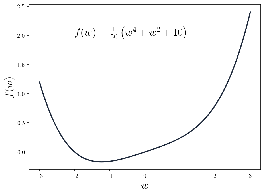
Finding the minimum with calculus

If you recall some calculus knowledge from high school, you can see that $f(w)$ is determined for all $w \in \mathbb{R}$, i.e., the function is continuous, so it has derivates at all points within its domain. The first-order and second-order derivates of the function are

As $f''(w) > 0$ for all $w \in \mathbb{R}$, we are convinced that $f$ is a convex function. Furthermore, as the function has both first-order and second-order deratives determined at all points, there exists points $w^*$ such that

and the function $f$ has its minimum at $w = w^*$. Since $f''(w) > 0$, to find $w^*$, we only need to solveI'm not going to devise the steps to solve this problem so that you will not feel that this article is about high-school calculus, not gradient descent. You can convince yourself here that $f'(w) = 0$ has a unique solutionThis is why I've told you it is unlikely to get the solution in 30 seconds if you do it by hands. Anyway, our function $f$ has a global minimum

Finding the minimum with gradient descent

Let's find the minimum of $f$ with gradient descent, and see if we would end up at the same solution above. Until now, I haven't told you what "convergence" means, so we modify our algorithm a bit by repeating the update step for $N$ times. Our algorithm now looks like this

We can implement this simple algorithm in Jax. Jax provides a convenient function grad to compute the gradient of an arbitarity function w.r.t. some input.

import jax.numpy as jnp
from jax import grad

# Define function f
def f(w):
  return 1/50 * (jnp.power(w, 4) + jnp.power(w, 2) + 10*w)

def gradient_descent(func, w, eta=0.1, n_iters=100):
  """
  Parameters:
  -----------
    func: the function we're minizing
    w : parameter we need to update
    eta: learning rate
    n_iters: number of iterations (N)
  """
  f_values, grad_values = []
  for _ in range(n_iters):
    grad_f = grad(func)(w)
    f_values.append(val_f)
    grad_values.append(grad_f)

    # Update step
    w = w - eta * grad_f

  return f_values, grad_values

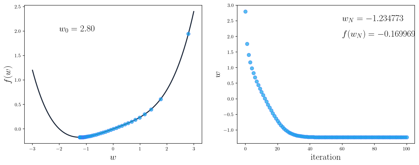
If we run the algorithm with $w_0 = 2.8, \eta = 0.5, N = 100$, and plot the values of the function $f$ and the estimated $w$, we would get something like this

If we run the algorithm again with a different $w_0 = -2.74$, we would get

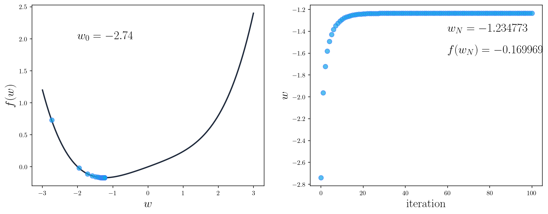
As you can see, in both cases, the parameter $w$ is updated so that $f(w)$ gradually moves toward its minimum. After the algorithm finishes, we arrive at a point $w = -1.2347723$ and $f(w) = -0.169969$ -- same as what we've got when finding the minimum using calculus.

Furthermore, we can see from the two plots on the right that after about $50$ iterations, the value of $w$ isn't changed anymore. This is when we say the algorithm has converged, meaning that no mater how long we continue the algorithm, the value of the parameter will stay the same. We can also see that in the first several iterations, gradient descent made big updates to $w$; however, as we crawl toward the optimal $w^*$, the updates become much smaller, very close to $0$ eventually.

General behavior of Gradient descent

• Gradient descent converges to a globcal minimum of a function if the function is convex. This is gauranteed regardless of the initialization $w_0$, learning rate, etc. provided that the function we're trying to minimize is convex.
• Gradient descent scales well with input dimension. Because we can apply gradient descent to each dimension of the input independently from other dimensions, the computation of gradient descent can be very efficient as the dimension of input grows.
• The learning rate $\eta$ should be chosen with care for gradient descent. In most problems involving neural networks and gradient descent, one should choose the step size $\eta$ of the algorithm carefully. Too small $\eta$ and the model won't learn anything useful and might not converge to any minimum. Too large $\eta$ and the model might get stuck, bouncing around a minimum but never actually ocvers to the minumum. We'll talk more about this phenomenon below.

Gradient descent and neural networks

The example above is a very simple and has unrealistic properties: our function $f$ is convex, we know its shape, and the parameter $w$ is only 1-dimensional. When working with deep neural networks, none of those propertities would ever be true. Indeed, deep neural networks are very complex, non-convex functions consisted of lots of non-linear transformations. We can't know the exact form of the function that the network is modelling and have to learn through data.

Training a neural network means to find its parameters to minimize some loss function $\mathcal{L}$. Gradient descent has been, by far, the most popular algorithm for updating weights of neural networks. Neural networks often have millions, or even billion parameters, and optimizing those parameters with gradient descent can be a nasty business.

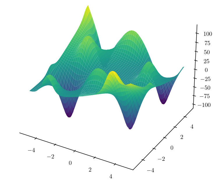
Problem 1: Local minimum

The picture above shows a more realistic loss function, and there exists multiple minimums called local minimum. Those are the points where our gradients are zero, but the value of the loss function at those points is not the smallest we can achieve. Since gradient descent is driven by gradient, if we start at some initial position, follow the direction of steepest descent of the gradient, we might very well end up at a local minimum, and our network can't really escape it.

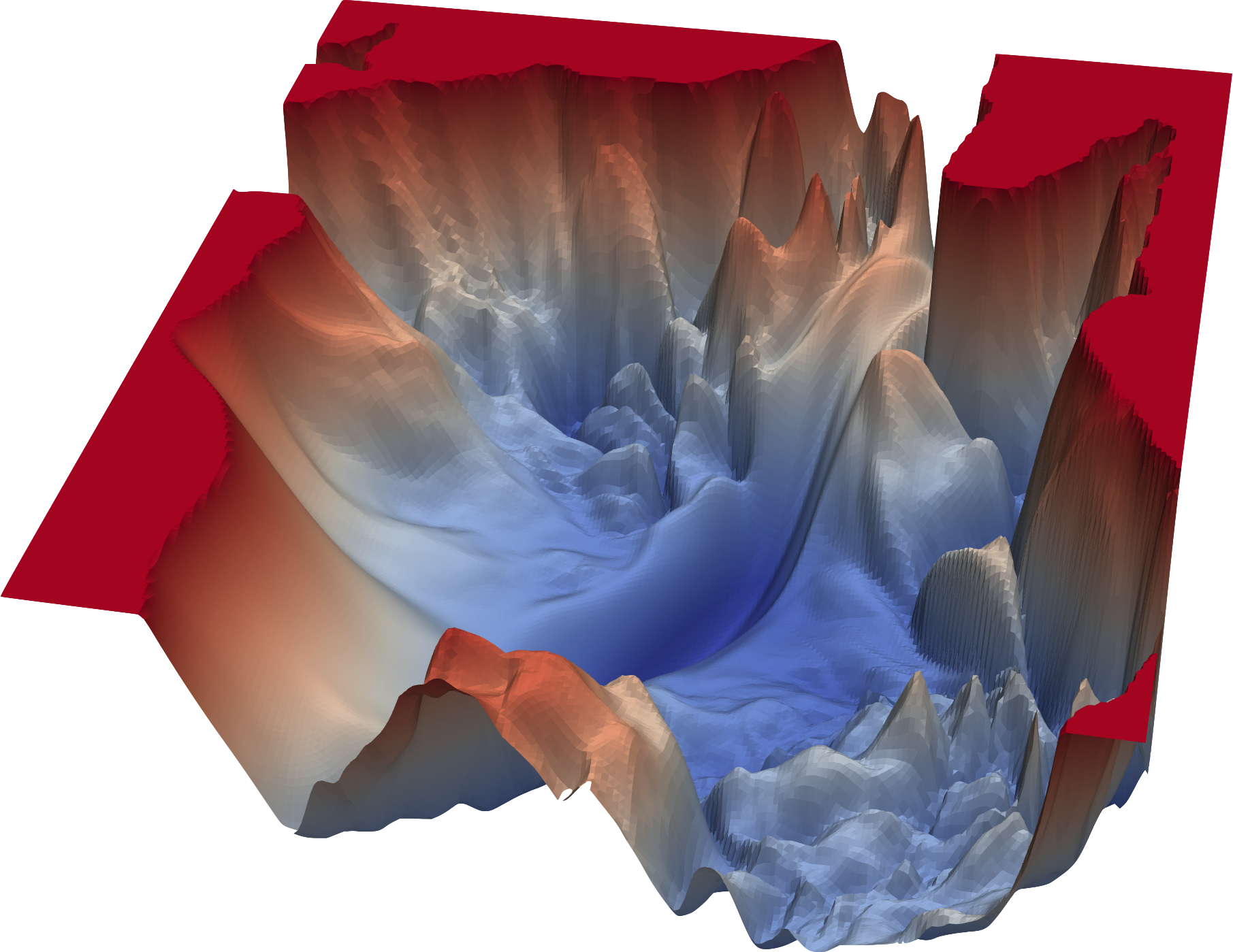
There has been an active line of research in understanding the loss landscape of neural networks. The picture below depicts a 3D visualization of a convolutional neural network (VGG-16) trained on the CIFAR-10 dataset. As you can see, the loss landscape is ridden with local minimums.

Problem 2: Saddle points

While local minimum is a challenge to gradient descent, it's not an inherent problem with the algorithm. The fact that gradient descent might not converge to a global minimum is because the loss function is not convex. Another problem inherent to gradient descent is called the saddle point problem.

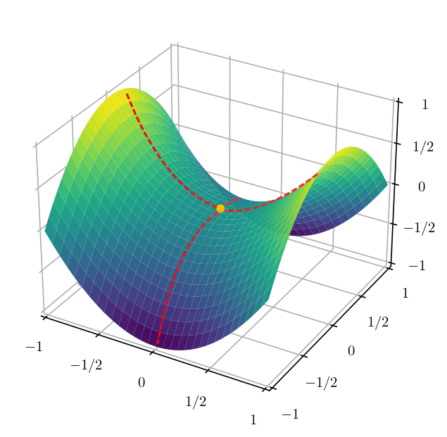
A saddle point is a point where it's minimum in one direction, and local maximum in another direction. If the loss landscape is flatten toward the mimimum direction, gradient descent will oscillate around the other direction – giving an illusion that the algorithm has convereged to a minimum.

Variants of gradient descent

Batch gradient descent

The description of gradient descent we've used so far in this article is actually called batch gradient descent. We compute the gradient for each parameter w.r.t the loss function for each training data point, and average the gradients across the dataset. Then we update all parameters at once, i.e., there is only one step of gradient descent at in epoch. This approach has two problems

• If we have a very large training dataset, which is oftent the case for deep neural networks, it might infeasible to compute the gradient of all training examples at once.
• As mention aboved, once we arrive at a local minimum, we are very likely to stuck there since all the parameters are updated using the same gradient, i.e., the avarage gradients across all training samples.

The rescue to those problems is to introduce randomness to the process.

Stochastic gradient descent

In this approach, instead of updating the parameter based on the gradient of all training examples, we update the parameter using the gradient computed from a single training example at each step, and we do this for all examples in our training dataset. In doing so, we introduce some sorts of randomness to the gradient descent. Indeed, we select one sample at a time, randomly, and calculate the gradient of the loss function w.r.t to the parameters. This gradient is an estimation of the actual gradient (computed on the entire dataset).

The pseudo-code for the algorithm can be rewritten as below

The gradient estimated from a single example might be slightly different from the actual gradient. Therefore, when the batch gradient desccent is stuck at some local minimum, stochastic gradient descent might steer the update in a slightly different direction, which helps us get out of that minimum region. Stochastic gradient descent (SGD) trades faster iteration speed for slow convergence since we have to do multiple update steps per epoch.

Mini-batch Stochastic Gradient Descent

It seems that SGD is a great improvement for batch gradient descent. But it also comes without drawbacks. Particularly, since we update the parameters based on gradient approximated by one example at a time, the learning might become too random and too slow. To remedy this problem, we choose an approach that is between all-example and one-example estimation, i.e., mini-batch gradient descent. The idea is that instead of estimating the gradient from one example, we do so from several example, i.e, a batch, at a time. And we have a new hyperparameter for our problem – batch size. The batch size is chosen to ensure some level of stochastity to cope with local minimum, while taking advantance of the parallelism in computing the gradient to reduce training time.

Summary

In this post, we go through gradient descent at high level, and how it can be used to train neural networks. Essentially, gradient descent has been the working horse for deep learning optimization. We've also talked about variants of gradient descent including batch, stochastic and mini-batch stochastic gradient descent. However, we did not touch some important topics when working with gradient descent, e.g., how sensitive it is to parameter initialization, the choice of lerning rate $\eta$, and the pathological curvature problem. They will be the topics for next post in ML4D series!

References

1. Gradient Descent, Machine Learning Refined. I borrowed the simple function $f$ from there.
2. Introduction to Optimization for Deep Learning: Gradient Descent, Paperspace
3. Stochastic Gradient Descent, Wikipedia