I do machine learning operation.
I'm an MLOps engineer with a love for software engineering, currently based in Stockholm.
I write about machine learning, software engineering and other things I've learned.
Recent posts
-
ArgoCD - The Fancy Local Setup
This guide walks you through setting up ArgoCD, in a local development environment using Minikube. The tutorial also covers making ArgoCD publicly acc...
devargocdminikubecloudflare -
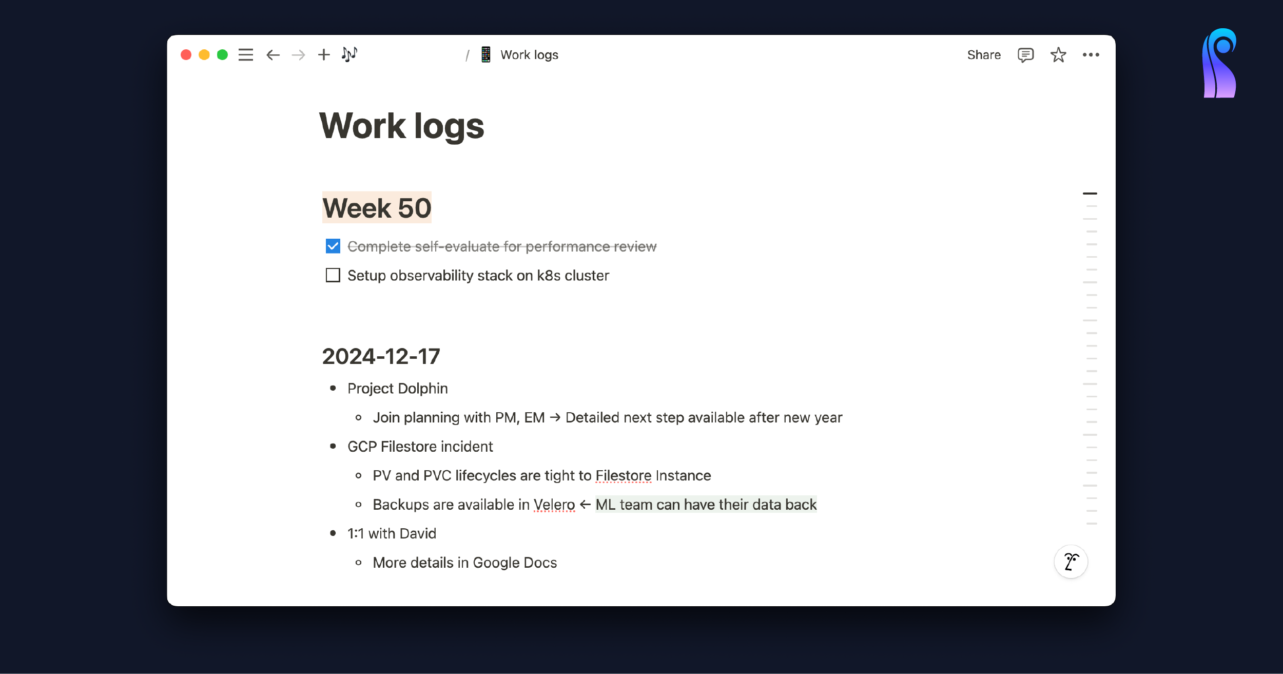
Benefits of a Work Log for Software Engineers
A work log is an efficient tool to track your progress, communicate more effectively, and gain a deeper understanding of your work. Plus, it serves as...
devcareer-growthmeta-learningproductivity -
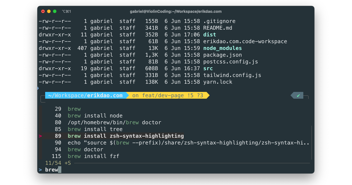
How to setup iTerm2 for development in 2024
If you're visiting this page, chances are that you're looking to make your iTerm2 even better, more beautiful and fun to work with. Let's dive in!
deviterm -
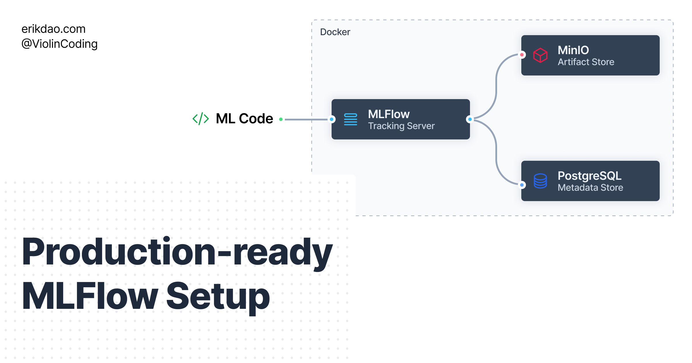
Production-ready MLFlow setup in your local machine
In this post, I'll show you how to setup a production-ready MLFlow environment in your local machine. The setup follows the remote tracking server sce...
machine learningmlops -

Gradient Descent
Gradient descent is an algorithm for finding the local minimum of a differential function by taking repated steps in the opposite direction of the gra...
ml4dmachine learninginterview prep -
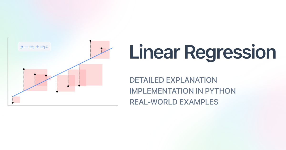
Linear Regression
Linear regression is the simplest method for regression analysis. With current state of machine learning and deep learning, we might often overlook li...
ml4dmachine learninginterview prep -
Evaluating Object Detection Models
In this article, we're going through several popular metrics used to evaluate the performance of object detection models for images.
machine learningobject detectionmetrics -

Simple Guidelines for Engineering Resumes
A resume is an essential component of your application package. Having a resume that concisely highlights your experience, skills, and potential contr...
life stories -

Bốn khoản chi phí "không tên" khi du học Thuỵ Điển
Việc lên kế hoạch tài chính, dự toán được những chi phí là rất cần thiết khi đi học ở một đất nước mới. Trong bài viết này, mình sẽ chia sẻ một số "hi...
life stories -

Khoản đầu tư 10 con số du học Thuỵ Điển
Du học tự túc là một khoản đầu tư lớn về thời gian, công sức và tiền bạc. Sau một năm học tập và sống tại Stockholm, mình đã có nhiều kinh nghiệm thực...
life stories